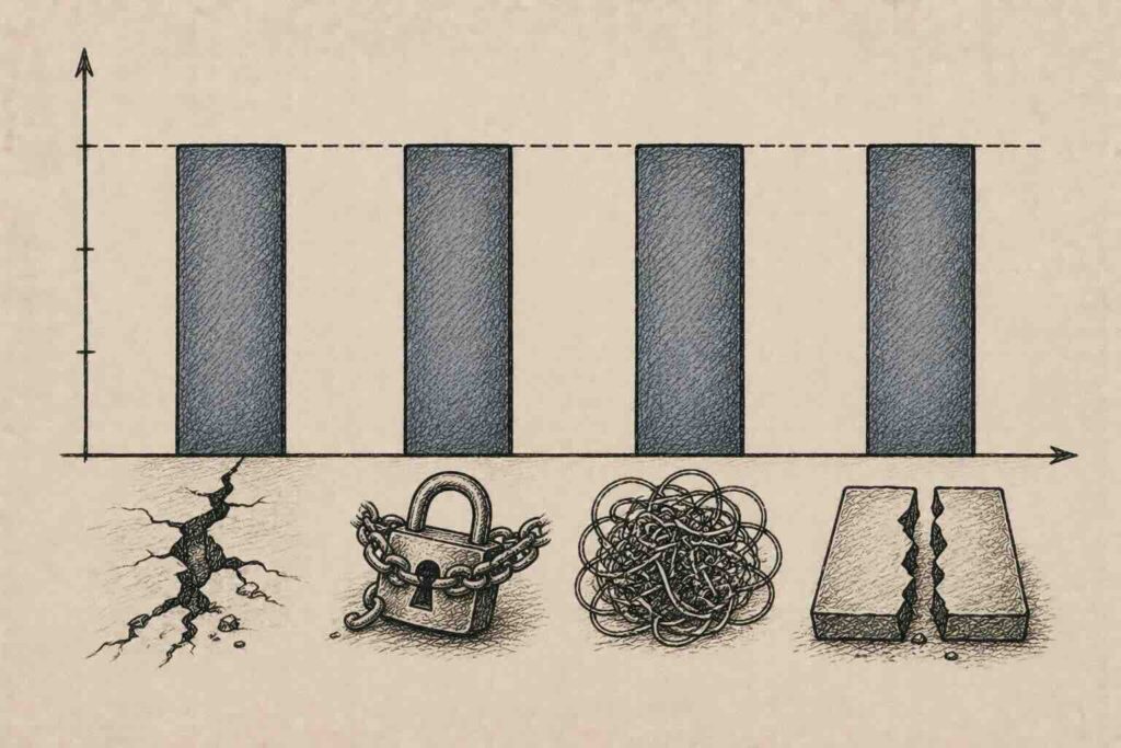
You are choosing a vector database, so you open the comparison charts. Most of them have one, and it tends to show the publisher on top. Queries per second, recall at some k, latency at some percentile, all plotted so the line with their name on it sits highest. You read a few of these and come away knowing less than when you started, because they do not disagree in any way that helps you. They are all fast. They are all accurate. They are all, at the sizes most teams run, more than good enough.
The charts converge because underneath they are optimizing the same thing. Choosing by that number is like ranking cars by top speed when you will spend every day in traffic. The number is real. It is just not the thing that will strand you.
The index is not the decision
Three of the four here expose HNSW directly, a proximity graph you search by hopping from node to nearby node until you arrive at the closest vectors. Think of it as a set of highways laid over your data, long edges at the top to cross the space quickly, dense short streets at the bottom to home in. It is approximate, it is fast, and the paper that defined it (Malkov and Yashunin, 2016) is cited across the field.
pgvector offers HNSW and IVFFlat and recommends HNSW for quality. Qdrant builds on HNSW and extends it. Weaviate defaults to HNSW. Pinecone is the deliberate exception: it exposes no index at all, and its own documentation says plainly that it has never used HNSW, automatically choosing proprietary algorithms by data size instead. You do not pick it, tune it, or even see it.
That variety is the point. Whether an engine runs an open HNSW graph you tune yourself or a proprietary index you never see, the published numbers land in the same range, because every one of them is optimized for the same recall-and-throughput game, and small differences come down to tuning, hardware, and which operating point someone chose to plot. Benchmark performance is the commodity. Everything that actually distinguishes these systems sits above the index, in how they filter, how they fuse keyword and vector search, how they isolate tenants, how they scale, and who pays when they do. A leaderboard cannot see any of that.
Why the benchmark cannot decide for you
There is one genuinely neutral benchmark worth knowing, ANN-Benchmarks, an open academic project that plots recall against throughput across standard datasets on the same hardware. It is careful and it is fair, and the useful part is that its own authors are explicit about what it does not measure. By their own account, the benchmark runs entirely in memory, on a single machine, over a static dataset with no inserts or deletes, one query at a time, and with no metadata filtering at all. Results are also highly sensitive to parameter tuning.
Read that list again, because it is the whole argument. The one fair, neutral benchmark deliberately excludes updates, distribution, and filtering, which are precisely the things that break in production. It measures the index in isolation under laboratory conditions and says nothing about the axes on which these databases actually differ. Even the honest number cannot tell you which database to run.
The vendor charts are worse, and it is worth naming why rather than trusting them. A vendor tuning its own system against a competitor's defaults, on a dataset and operating point it selected, publishing the run where it wins, is not producing evidence. It is producing marketing. There are enough of these charts with mutually incompatible winners that the genre cannot settle the decision for you. I am not going to quote their numbers, because the numbers are the wrong question.
The question the benchmark hides: filtered search
Here is a question no leaderboard answers, and it is the one that will actually hurt you. You do not usually want the nearest vectors. You want the nearest vectors where something is true: this user's documents, in stock, published after a date, in a language. That is filtered vector search, and it is one phrase hiding two different ways to fail.
You can filter after searching. Find the nearest k vectors, then drop the ones that fail the condition. The trap is that a selective filter can discard almost the entire result set. pgvector's own documentation gives the concrete case: with the default search settings, a filter that matches ten percent of rows leaves, on average, about four results out of the top forty, even though plenty of matching vectors exist elsewhere in the table. They just were not in the first similarity pass. Your recall silently collapses, and nothing errors.
Or you can filter before searching, restricting the graph to only the vectors that pass. That breaks the other way. HNSW navigates by its edges, and if you delete most of the nodes, the highways that made search fast may run through vectors you just excluded. Traversal gets stranded and never reaches valid matches. Same query, opposite failure.
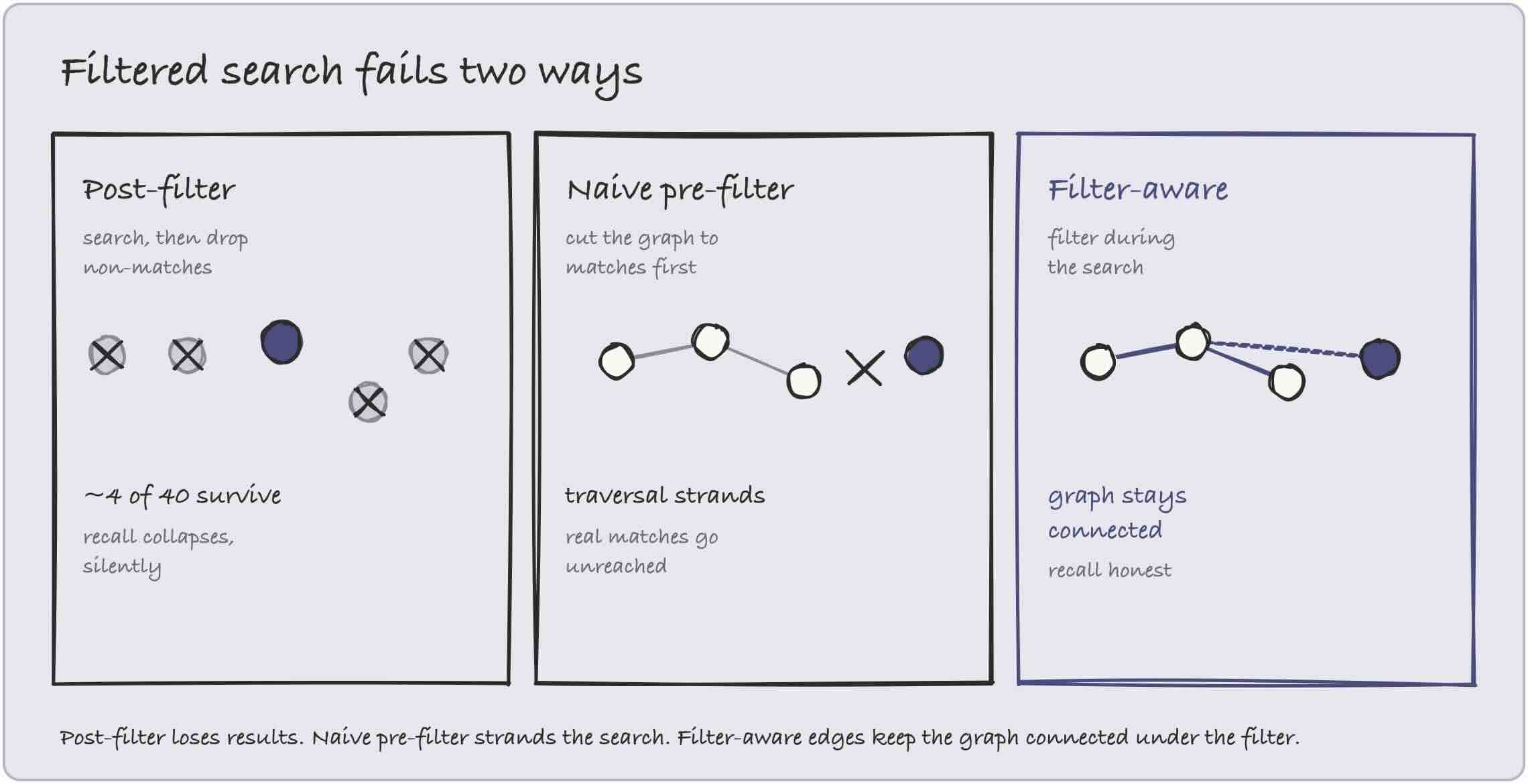
This is where the engines genuinely diverge, and it is invisible on any benchmark because ANN-Benchmarks does not filter at all. Qdrant treats this as its defining problem: its filterable HNSW adds extra edges to the graph based on indexed metadata values, so a filtered subset stays connected and traversable, with a planner that falls back to an exact scan when the filter is selective enough that the graph is not worth it. The cost is that, for the fields you want that filterable-HNSW behavior on, you declare those payload indexes up front, before you load data. pgvector mitigates its post-filter problem with iterative index scans, added in version 0.8.0, which keep scanning more of the index when the filter drops too many rows. Pinecone folds the filter into the query engine as a single stage rather than a cleanup pass afterward. Weaviate filters during the search against an inverted index. Four engines, four different answers to a question the benchmark never asks.
Four engines, four failure modes
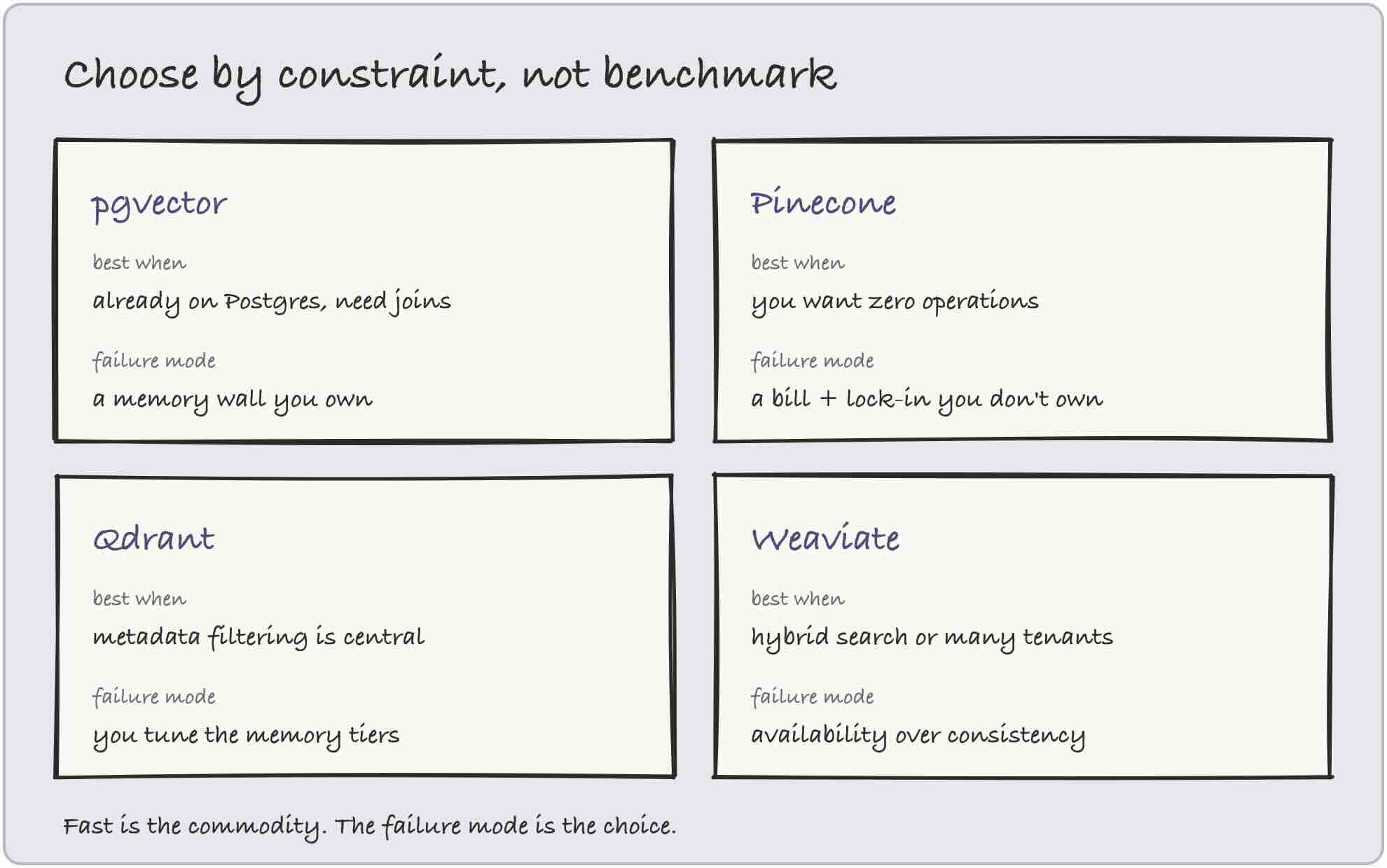
Once you stop ranking by speed, each database resolves into a distinct shape: the constraint it is built for, and the failure you inherit in return. That is the honest way to choose, by deciding which failure you can live with.
pgvector is a vector column inside Postgres. Not a separate system, an extension. Your vectors sit in a table next to your relational data, with the same transactions, joins, backups, and replication you already run, and a search is just a SQL query with an ORDER BY on distance. If you are already on Postgres, this is close to free operationally, and you can filter and join vectors against real business tables in one transaction. The failure mode is a wall you own. HNSW wants to live in memory, and that memory competes with your transactional workload on the same box. There is no native horizontal scale-out; past a single large node you are bolting on external sharding or migrating. It is the right answer under moderate scale and relational gravity, and the wrong one when the index outgrows the machine.
Pinecone is a managed serverless service. Storage and compute are decoupled, the index type is chosen and tuned by Pinecone rather than by you, and there is nothing to provision, size, or operate. It is the fastest path from nothing to a working index, which is a real advantage when you have no infrastructure team and no desire to become one. The failure mode is the mirror image of pgvector's: you do not own the wall, but you do not own the levers either. Cost is metered by usage, reads and writes and storage, so a sustained high-query workload converts directly into a bill that a fixed server would have capped, and there is no self-host escape hatch because the system is proprietary. You trade operational control and cost predictability for having no operations at all. When the bill or the lock-in becomes the problem, there is no knob you own to turn.
Qdrant is a filtering-first engine. Written in Rust, built around the filterable HNSW described above, with rich payload conditions (ranges, geo, datetime, full text on metadata) and fine control over how much of the index lives in RAM versus memory-mapped on disk. If your queries are fundamentally "nearest vectors where a lot of conditions hold," this is the engine that keeps recall honest under those filters instead of quietly dropping results. The failure mode is that the control is yours to manage: you declare payload indexes before ingest, and you tune the memory tiers, quantization, and consistency factors yourself. It is the right answer for filter-heavy retrieval, and more engine than you need if your filtering is light.
Weaviate is built for hybrid search and multi-tenancy. Its hybrid search fuses keyword (BM25) and vector results as a first-class query with a single alpha knob to bias lexical versus semantic, which matters whenever exact terms like part numbers or names must not be lost to pure semantic similarity. Its multi-tenancy gives each tenant its own shard and an active, inactive, or offloaded state, so a SaaS with a million customers can keep only the active ones in memory and park the rest on cheap storage. The failure mode lives in its defaults: the data path favors availability over consistency, so under a partition it will serve a possibly stale read rather than refuse, and holding HNSW in memory means you tune indexes and compression to keep the footprint sane. It is the right answer for hybrid relevance and multi-tenant SaaS, and it asks you to mind consistency and memory in return.
| Engine | What it is | Best when | The failure mode you accept |
|---|---|---|---|
| pgvector | A vector column inside Postgres | You already run Postgres and need joins and transactions on your data | A single-node memory wall you own; the index competes with your database |
| Pinecone | Managed serverless, storage and compute decoupled | You want time-to-production and no operations | A metered bill and lock-in you do not control |
| Qdrant | Filtering-first engine (filterable HNSW) | Metadata filtering is central to your queries | You pre-declare indexes and manage memory tiers yourself |
| Weaviate | Hybrid search and first-class multi-tenancy | You need keyword-plus-vector fusion, or many isolated tenants | An availability-first data path you tune for consistency |
The axes that actually decide
Notice what did the work in that table. Not one of the distinctions was a speed number. They were architectural axes, and on almost every one the best choice flips depending on your constraint.
Filtering points to Qdrant. Hybrid keyword-and-vector search points to Weaviate, though Qdrant and Pinecone support it too. Multi-tenancy at real scale points to Weaviate's per-tenant shards or Pinecone's namespaces. Least operational burden points to Pinecone. Cost points wherever your usage pattern is cheapest: marginal on an existing Postgres bill for pgvector, metered and cheap-when-idle for Pinecone, or a fixed machine you size for peak with self-hosted Qdrant and Weaviate. And the axis no benchmark will ever contain: where you already are. If your vectors need to be joined and filtered against relational data you already keep in Postgres, adding a second specialized store buys you ANN performance you may not need at the price of a synchronization problem you definitely do not want.
Re-indexing cost belongs on this list too, because it compounds the operational choice. Changing your embedding model forces you to rebuild the entire index, and how painful that is depends entirely on which of these systems you are running it on.
The pattern underneath
A benchmark is a declared number. It is the system telling you how it performs under conditions someone chose. Production is the observed behavior, how the system fails when the filter is selective, when the tenant count climbs, when the bill arrives, when the model changes and everything must be rebuilt. The gap between those two is the same gap that runs under most of this work, the difference between what a system reports about itself and what it actually does. The benchmark is the declared state. The failure mode is the observed one, and it is the one you live with.
So the comparison that matters is not which engine wins the chart. It is which way each one fails, and whether that failure is one your team, your scale, and your budget can absorb. All four are fast. That was never in doubt, and it was never the question.
They are all fast. Fast is the commodity. What you are actually choosing is a failure mode.
Sources
The figures here are reported by the vendors and papers cited, each on their own evaluation and documentation, not independently verified. Read them as directional.
- Malkov & Yashunin, "Efficient and robust approximate nearest neighbor search using Hierarchical Navigable Small World graphs," IEEE TPAMI 2020 (arXiv 1603.09320).
- Aumüller, Bernhardsson & Faithfull, "ANN-Benchmarks: A Benchmarking Tool for Approximate Nearest Neighbor Algorithms," Information Systems 2020 (arXiv 1807.05614); ann-benchmarks.com.
- Qdrant, "A Complete Guide to Filtering in Vector Search" and the indexing documentation (filterable HNSW, payload indexes).
- pgvector documentation (HNSW and IVFFlat, post-filter behavior, iterative index scans in 0.8.0).
- Pinecone documentation: "Pinecone's Indexing Algorithms" (states it has never used HNSW; auto-selects proprietary algorithms by data size) and the serverless architecture reference (single-stage metadata filtering, usage-based pricing; figures reported by the vendor).
- Weaviate documentation on hybrid search and multi-tenancy, and its replication architecture (availability-first data path).