Introduction: Diving into the World of Neural Networks
Welcome aboard, folks! We're about to embark on a thrilling journey into the world of neural networks - an integral part of the exciting machine learning and deep learning landscape.
What is a Neural Network?
Imagine your brain. Now imagine it a lot simpler (no offense intended!). That's what a neural network is, in essence. A neural network is a computing system inspired by the human brain. It's made up of interconnected nodes, or 'neurons', organized in layers, that work together to solve specific problems.
It's a bit like a team of detectives, each focusing on a different aspect of a case and pooling their findings to crack it. Each neuron processes input, applies a transformation (usually nonlinear), and passes the output to the next layer - just like a diligent detective passing their clues along the chain.
Importance of Neural Networks in Machine Learning and Deep Learning
Neural networks are the beating heart of deep learning, which is a subfield of machine learning.
Why are they important? Well, there are a few reasons:
- Universality: Neural networks can approximate pretty much any function given enough neurons and layers, which makes them super versatile. They're like the Swiss army knife of machine learning!
- Handling Complex Data: Neural networks excel at handling unstructured and complex data, like images, audio, and text. They're great at finding hidden patterns and structures in these data types, kind of like a truffle pig on a hunt.
- End-to-End Learning: Neural networks can learn directly from raw data without needing manual feature extraction, which can be a huge time saver. It's like going directly from farm to table!
So, buckle up, and get ready for an exciting exploration of neural networks - the all-star team of deep learning!
Basic Components of a Neural Network
Like a high-tech gadget, a neural network is made up of several components that work together in harmony. Let's roll up our sleeves and take a peek under the hood.
Neurons
First, we have neurons, the fundamental building blocks of a neural network. These little guys take in input, do some computation, and produce output. Picture them as tiny problem solvers, each contributing a small part to the bigger solution.
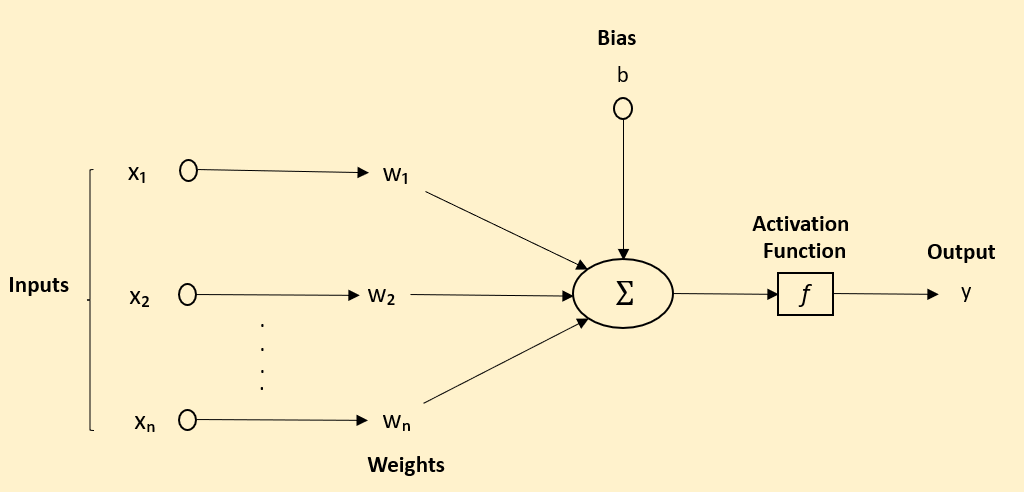
Here x is the input vector, w is the weight vector, and b is the bias. The function f is the activation function.
Weights and Biases
Next up, weights and biases - the dynamic duo that fine-tunes the output of our neurons. Weights adjust the influence of each input, while biases allow us to shift the activation function to fit the data better. They're the knobs and dials that we tweak during training to improve our neural network's performance.
Activation Functions
Activation functions are the magic transformation spells of the neural network world. They decide how much signal should pass from one layer to the next. Some, like ReLU (Rectified Linear Unit, are like bouncers at a club, only letting through the positive vibes (or in this case, values). Others, like the sigmoid function, squash everything between 0 and 1, providing a probabilistic output.
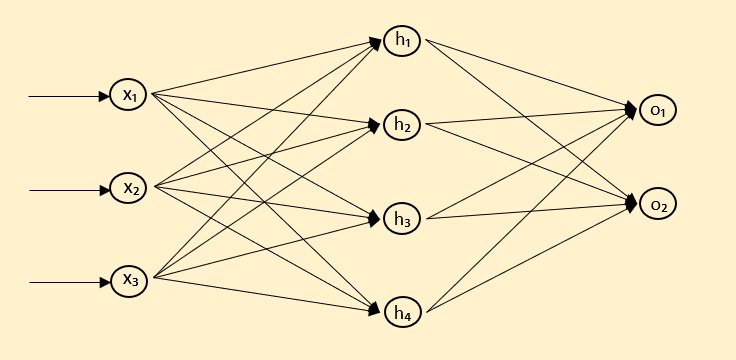
Layers: Input, Hidden, and Output
A neural network is typically composed of three types of layers:
- Input Layer: This is the layer that receives the raw data. It's like the doorman, taking your coat (data) as you enter the network.
- Hidden Layers: These are the layers in between input and output. They do the heavy lifting of learning from the data. Picture them as a bustling kitchen, transforming raw ingredients (data) into a mouthwatering meal (useful insights).
- Output Layer: This is the final layer that presents the results. It's the waiter serving up the dish (the network's final output).
Together, these components form a versatile machine that can learn from data and make smart predictions. Welcome to the wondrous world of neural networks - it's going to be a fantastic ride!
Working of a Neural Network
Ready to take a closer look at how neural networks work their magic? Good! We've got quite a journey ahead. It's a two-step dance: Forward Propagation and Backward Propagation, with a sprinkle of Loss Functions, Gradient Descent, and Optimizers. Let's get moving!
Forward Propagation:
Each layer takes the outputs of the previous layer (or the input data for the first layer), applies the weights, adds the bias, and then applies the activation function. This is then passed as input to the next layer. Let's say we have a single neuron for simplicity. The output y of the neuron for an input x is calculated as:
z = Wx + b (where W is the weight matrix and b is the bias vector)
y = f(z) (where f is the activation function)
We do this for each layer until we reach the output layer. The final output is our network's prediction based on the input data.
Backward Propagation:
After forward prop has had its turn, backward propagation steps in.
During backward propagation, we start by comparing the output of the network (from forward propagation) to the expected output, using a loss function. The Loss Function is our reality check. It tells us how far off our predictions are from the actual values. It's like a coach, pointing out where we went wrong. During backward propagation, we aim to adjust our weights and biases to minimize this loss. The result is an error value that we want to minimize.
Loss = L(y, y_hat) (where L is the loss function, y is the actual output and y_hat is the network's predicted output)
Then we use this error to calculate gradients for all the weights and biases in the network, which tell us how to change the parameters to reduce the error. This is done using the chain rule of differentiation, hence the name backpropagation.
The formula for the weight update is:
W = W - α * dL/dW
Here, α is the learning rate (a small step size), and dL/dW is the gradient of the loss function with respect to the weights. The bias update is similar.
Backpropagation continues layer-by-layer from the output layer back to the input layer, updating all the weights and biases along the way based on their contribution to the error.
And that's the basic idea of forward and backward propagation! It's like a well-choreographed dance between all the parts of the neural network, each doing its part to create the final result. Keep on learning, and soon you'll be choreographing your own neural network performances!
Types of Neural Networks
Neural networks come in all shapes and sizes, much like the animals in a zoo. From the humble Feedforward Neural Networks, the 'goldfish' of our neural network zoo, to the more exotic Convolutional Neural Networks, the 'tigers'. Let's visit them!
Feedforward Neural Networks
Feedforward Neural Networks are the OGs of the neural network world. Simple and reliable, they get the job done. As the name suggests, the information in these networks travels in one direction - from the input layer, through the hidden layers, and out the output layer. It's like a one-way street, no U-turns allowed!
FNNs are the foundation of most neural networks, and they're great for a wide range of tasks, from classifying emails (spam or not-spam) to predicting house prices.
# Here's a quick example of a feedforward neural network using Keras
from keras.models import Sequential
from keras.layers import Dense

# Create a Feedforward Neural Network with one hidden layer
model = Sequential([
    Dense(10, input_dim=8, activation='relu'),
    Dense(1, activation='sigmoid')
])

# Compile the model
model.compile(loss='binary_crossentropy', optimizer='adam', metrics=['accuracy'])
Convolutional Neural Networks (CNNs)
Next, let's turn to the visual whiz kid of the family, the Convolutional Neural Network. CNNs have an uncanny ability to handle image data. They're the secret sauce behind most of the fancy image recognition tech you see today, from face recognition in your phone's photo gallery to self-driving cars.
The 'convolutional' in their name comes from the mathematical operation called 'convolution' that they use to filter inputs for useful information. They have this nifty structure that mimics how our human visual cortex works.
A CNN typically consists of three types of layers: convolutional layers, pooling layers, and fully-connected layers. Convolutional layers apply a series of filters to the input. Pooling layers then reduce the spatial dimensions (height, width), keeping the most important information. Finally, fully-connected layers take this high-level information and output a prediction.
To put it in human terms, imagine recognizing a friend (let's call him Bob). First, you notice basic features like colors and edges (that's the convolutional layer). Then, you identify parts of Bob like his nose, eyes, or hair (that's the pooling layer). Finally, you put it all together and shout, "Hey, that's Bob!" (that's the fully-connected layer).
# Let's create a simple Convolutional Neural Network using Keras
from keras.models import Sequential
from keras.layers import Conv2D, MaxPooling2D, Flatten, Dense

# Create a CNN with one convolutional layer
model = Sequential([
    Conv2D(32, (3, 3), activation='relu', input_shape=(64, 64, 3)),
    MaxPooling2D(pool_size=(2, 2)),
    Flatten(),
    Dense(128, activation='relu'),
    Dense(1, activation='sigmoid')
])

# Compile the model
model.compile(optimizer='adam', loss='binary_crossentropy', metrics=['accuracy'])
Recurrent Neural Networks (RNNs)
Recurrent Neural Networks, or RNNs, are the social butterflies of neural networks. Unlike their Feedforward cousins who process each input independently, RNNs remember. They keep track of previous inputs in their hidden layers, creating a kind of 'internal memory'. This makes them fabulous for handling sequential data, like time series or natural language, where the order of inputs matters.
Imagine trying to understand this sentence without remembering the previous words - pretty hard, right? That's what RNNs excel at!
# Here's a simple example of an RNN using Keras
from keras.models import Sequential
from keras.layers import SimpleRNN, Dense

# Create a RNN with one recurrent layer
model = Sequential([
    SimpleRNN(10, input_shape=(None, 1)),
    Dense(1)
])

# Compile the model
model.compile(optimizer='adam', loss='mean_squared_error')
Long Short-Term Memory Networks (LSTMs)
But RNNs have a downside - they tend to forget things after a while, especially in long sequences. Enter Long Short-Term Memory Networks, or LSTMs, the elephants of the neural network zoo. LSTMs are a special kind of RNN, designed to remember long-term dependencies in data. They can remember or forget information using special structures called gates.
If RNNs are like a group of friends trying to remember a story, LSTMs are like that friend with the photographic memory who can recall every little detail from years ago. They're the go-to choice for complex sequence problems, like machine translation or speech recognition.
# And now an LSTM using Keras
from keras.models import Sequential
from keras.layers import LSTM, Dense

# Create an LSTM with one LSTM layer
model = Sequential([
    LSTM(50, input_shape=(None, 1)),
    Dense(1)
])

# Compile the model
model.compile(optimizer='adam', loss='mean_squared_error')
Autoencoders
Autoencoders are the minimalists of the neural network world. Like an artist who distills a landscape into a few simple brush strokes, an autoencoder learns to compress input data into a simpler (lower-dimensional) form, then reconstructs it as closely as possible. They're a type of unsupervised learning method - they learn from the input data without needing any labels.
They're great for tasks like noise reduction or anomaly detection, where learning the 'normal' state of the data can help identify the 'abnormal'.
# Here's a simple example of an autoencoder using Keras
from keras.models import Model
from keras.layers import Input, Dense

# The size of encoded representations
encoding_dim = 32

# Input placeholder
input_img = Input(shape=(784,))

# Encoded representation of the input
encoded = Dense(encoding_dim, activation='relu')(input_img)

# Reconstruction of the input
decoded = Dense(784, activation='sigmoid')(encoded)

# Model that maps an input to its reconstruction
autoencoder = Model(input_img, decoded)

# Compile the model
autoencoder.compile(optimizer='adadelta', loss='binary_crossentropy')
Generative Adversarial Networks (GANs)
GANs are the dramatic duos of the neural network world. They're composed of two separate networks: a generator and a discriminator. The generator creates new data instances, while the discriminator evaluates them for authenticity. It's like a game of cat and mouse, where the generator (the mouse) tries to fool the discriminator (the cat), and the discriminator tries to catch the generator out.
They're great for generating new data that resembles your existing data. Fancy generating new artwork in the style of Picasso? Or creating new levels for a video game? GANs are your go-to!
Training a Neural Network
Training a neural network isn't all fun and games. It's like teaching a dog new tricks, but instead of "Sit!" or "Fetch!", we're teaching our neural network to, say, distinguish cats from dogs in photos or predict tomorrow's weather. Let's dive right into the nitty-gritty details!
Dataset Splitting (Training, Validation, Test)
The first thing we need to do is split our dataset into three parts: training, validation, and test sets. Imagine you're studying for a big test. You learn from textbooks (training set), practice with quizzes (validation set), and then the final examination (test set) comes around. That's exactly how our neural network learns too!
# Here's a simple example of splitting a dataset using sklearn
from sklearn.model_selection import train_test_split

# Assuming X is your data and y are your labels
X_train, X_temp, y_train, y_temp = train_test_split(X, y, test_size=0.3)  # 70% training, 30% temporary
X_val, X_test, y_val, y_test = train_test_split(X_temp, y_temp, test_size=0.5)  # split temporary set into validation and test
Overfitting, Underfitting, and Techniques to Address Them
Now, while training our neural network, we might encounter the infamous duo of Overfitting and Underfitting.
Overfitting is when our neural network becomes an 'ace student', but only for the training set. It learns the training data so well, including its noise and outliers, that it performs poorly on unseen data. It's like studying only from one textbook and failing to answer questions from any other source.
On the other hand, Underfitting is when our neural network is the 'lazy student' who doesn't study enough to understand even the training set, let alone the validation or test set.
To deal with overfitting, we've got a couple of techniques up our sleeve like regularization (adding a penalty term in the loss function) and dropout (randomly ignoring some neurons during training to avoid reliance on any one feature).
# Example of a simple dense layer with dropout and L1 regularization
from keras.layers import Dense, Dropout
from keras import regularizers

model.add(Dense(64, input_dim=64,
                kernel_regularizer=regularizers.l1(0.01),
                activity_regularizer=regularizers.l1(0.01)))
model.add(Dropout(0.5))  # Dropout rate of 0.5
For underfitting, we might need to make our model more complex, like adding more layers or neurons, or we might need to train it for a longer time. And if all else fails, consider revisiting your data. Garbage in, garbage out, as we say!
Regularization Techniques: Dropout, L1/L2 Regularization
Dropout is like the Russian roulette of the neural network world. During training, it randomly "drops out" or deactivates some neurons in a layer, which forces the network to learn more robust features. It's like telling your neural network, "Hey, you can't rely on that one smart neuron all the time, you've got to distribute the workload!"
# Implementing dropout in Keras is a piece of cake
from keras.layers import Dropout

model.add(Dropout(0.5))  # Dropout rate of 0.5
L1/L2 Regularization are our network's personal trainers, keeping them from getting 'overweight' with large coefficients that might lead to overfitting. L1 can also help with feature selection, as it tends to produce sparse vectors. L2, on the other hand, doesn't favor sparse vectors but can help in preventing outlier features from having too much influence.
# Adding L1/L2 regularization in Keras is straightforward too
from keras import regularizers

model.add(Dense(64, input_dim=64,
                kernel_regularizer=regularizers.l1(0.01)))  # L1 regularization
model.add(Dense(64, input_dim=64,
                kernel_regularizer=regularizers.l2(0.01)))  # L2 regularization
Tuning Hyperparameters
Hyperparameters are like the dials and knobs on a sound mixer. They control everything from how fast the network learns (learning rate), to how much memory it has (number of layers and neurons), and how much the network can forget (dropout rate, regularization parameters).
Finding the right set of hyperparameters can feel like looking for a needle in a haystack. Thankfully, we have techniques like Grid Search and Random Search, or more advanced methods like Bayesian Optimization.
# Using Grid Search with Keras wrapper for hyperparameter tuning
from keras.wrappers.scikit_learn import KerasClassifier
from sklearn.model_selection import GridSearchCV

def create_model(optimizer='adam'):
    model = Sequential()
    model.add(Dense(12, input_dim=8, activation='relu'))
    model.add(Dense(1, activation='sigmoid'))
    model.compile(loss='binary_crossentropy', optimizer=optimizer, metrics=['accuracy'])
    return model

# create model
model = KerasClassifier(build_fn=create_model, epochs=100, batch_size=10, verbose=0)

# define the grid search parameters
optimizer = ['SGD', 'RMSprop', 'Adagrad', 'Adadelta', 'Adam', 'Adamax', 'Nadam']
param_grid = dict(optimizer=optimizer)

grid = GridSearchCV(estimator=model, param_grid=param_grid, n_jobs=-1, cv=3)
grid_result = grid.fit(X, Y)
Tuning a neural network might seem daunting, but remember, it's all about trial and error. You can't find the perfect sound without tweaking the mixer a bit.
Practical Application of Neural Networks
Alright folks, it's showtime! You've slogged through the theory, you've battled with backpropagation, and you've triumphed over training. Now, let's see where all this neural network jazz really shines - in the real world!
Real-world Use-cases
- Image Recognition: Neural networks are like modern-day Picassos. They're brilliant at recognizing and classifying images. Whether it's spotting a cat in your photo album, identifying tumors in medical scans, or powering self-driving cars, image recognition has endless possibilities. Convolutional Neural Networks (CNNs) are typically the stars of this show.
- Natural Language Processing (NLP): Ever chatted with Siri, Alexa, or any other AI assistant? That's all thanks to neural networks' ability to understand, interpret, and generate human language. From translation services to sentiment analysis, NLP is a hotbed of activity. Recurrent Neural Networks (RNNs) and Transformers often steal the spotlight here.
- Recommendation Systems: Netflix's "Recommended for You" or Amazon's "Customers Who Bought This Also Bought" features are powered by neural networks. They analyze your behavior and preferences to suggest products or services you might like. Usually, a special kind of autoencoder or a deep learning variant is behind the curtain.
- Anomaly Detection: Neural networks can spot when things are 'not quite right'. From detecting fraudulent transactions in real-time to identifying machine failures before they happen, anomaly detection is a major application area.
Success Stories
- Google Translate: This nifty tool uses a type of RNN called LSTM (Long Short-Term Memory) to translate between 100+ languages. It's like having a personal UN translator in your pocket!
- DeepMind's AlphaGo: It stunned the world by defeating the world champion in the complex game of Go. It used a combination of CNNs and reinforcement learning, a technique that lets neural networks learn from their mistakes, kinda like how you'd train a puppy.
- Facebook's DeepFace: It can recognize faces with an accuracy of 97.35%, which is pretty much on par with human performance. So the next time Facebook tags you in a photo, remember to say thanks to the deep learning models working behind the scenes.
Challenges in Designing and Training Neural Networks
Even with all their superpowers, neural networks have their kryptonite. Let's take a walk on the wild side and peek into some challenges you might face when taming these neural beasts.
Vanishing/Exploding Gradients
First up, the infamous "Vanishing/Exploding Gradients" problem. It sounds like something out of a sci-fi movie, but it's very real and can be a total party pooper. Let's break it down:
Vanishing gradients: As we go back in time (during backpropagation), gradients often get smaller and smaller. Eventually, they become so tiny, they're almost zero. This means the weights and biases of the initial layers don't get updated effectively. The result? A network that's about as useful as a chocolate teapot.
Exploding gradients: The evil twin of vanishing gradients. Here, the gradients become so large, they're off the charts. This can cause your model to overshoot the optimal solution in training. Imagine trying to make a gentle turn, but you end up doing donuts instead!
Luckily, there are ways to combat these issues. Initialization techniques like He or Xavier, activation functions like ReLU, and techniques like gradient clipping and batch normalization are like the Avengers to these villainous gradients.
Computational Requirements
Next on our challenge parade is the often overlooked, yet brutal, "Computational Requirements". Neural networks, especially the deep ones, have a big appetite for computational resources.
Training large neural networks requires an army of neurons and layers, and each of them demands its share of computations. This can be a real pain, especially if you're working on a standard laptop that heats up at the mere mention of 'deep learning'.
And then there's the memory. Storing the intermediate values for each neuron during forward propagation (for later use in backpropagation) can eat up a lot of memory. In the worst case scenario, your machine may run out of memory and crash, turning your deep learning dream into a nightmare!
Some solutions to this include using more efficient hardware (think GPUs, TPUs), optimizing your code, or turning to cloud-based platforms that offer scalable compute power. Pruning and quantization are also clever techniques to reduce the computational cost without sacrificing too much on performance.
So yes, neural networks can be a bit of a drama queen. But with patience, smart strategies, and a good sense of humor, you'll be just fine. Remember, every superhero has its challenges - it's overcoming them that makes the story worth telling!
Conclusion
As we reach the finish line of this neural journey, let's take a moment to reflect. Neural networks are like intricate, electronic brains. They can do amazing things, from recognizing your doodles to powering self-driving cars. They're exciting, they're revolutionary, and they're just plain cool.
But remember, this field is as dynamic as a gymnast on a sugar rush. New research papers pop up faster than popcorn kernels in a microwave. Models that were the cat's pajamas yesterday might be old hat tomorrow.
So, what's the secret to staying afloat in this sea of constant change? It's simple - never stop learning. Be like a sponge, ready to absorb all the knowledge you can. Stay curious. Ask questions. Tinker. Experiment. Fail. Learn. Repeat.
Sure, it might be a bit overwhelming at times. You might feel like you're chasing a moving target while juggling flaming torches. But hey, no one said being a machine learning engineer would be a cakewalk!
So, keep up with the latest research, join a community, attend workshops and webinars, engage in online forums, and most importantly, keep that enthusiasm alive. Python and its machine learning libraries are your trusty sidekicks in this journey.
Learning is a lot like rowing upstream. If you stop, you drift back. So keep rowing, keep learning, and remember to have a blast while doing it!
Stay tuned for our next blog post where we will dive into another exciting aspect of machine learning.
References
Feed Forward Neural Network using Keras
Convolutional Neural Networks using Keras
Recurrent Neural Networks using Keras