Linear Regression is the most commonly used predictive analysis. It is used to model the relationship between a dependent variable and one or more independent variables. In this project we create an ML pipeline to train a linear regression model to predict the release year of a song given a set of audio features. We implemented this project on Apache Spark 1.6.1 on databricks cloud platform. We used subset of the Million Song Dataset from the UCI Machine Learning Repository
The first value in the data is label and the rest are the features.
file_name = '/databricks-datasets/cs190/data-001/millionsong.txt'
raw_data_df = sqlContext.read.load(file_name, 'text')
print raw_data_df.show()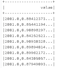
In MLlib, labeled training instances are stored using the LabeledPoint object. So, we write a function that takes in a DataFrame and parse each row in the DataFrame into a LabeledPoint.
def parse_points(df):
  """Converts a DataFrame of comma separated unicode strings into a DataFrame
     of LabeledPoints.

  Args:
    df: DataFrame where each row is a comma separated unicode string. The first element
    in the string is the label and the remaining elements are the features.

  Returns:
    DataFrame: Each row is converted into a `LabeledPoint`, which consists of a label and
               features.
  """
  return (df.select(sql_functions.split(df.value, ',')).alias('value')
          .map(lambda row: LabeledPoint(float(row[0][0]), list(row[0][1:])))
          .toDF(['features', 'label']))
Now we split the dataset into training, validation and test sets. Once that is done we cache each of these datasets because we will be accessing those multiple times.
weights = [.8,.1,.1]
seed= 23
parsed_train_data_df, parsed_val_data_df, parsed_test_data_df = parsed_data_df.randomSplit(weights, seed)
parsed_train_data_df.cache()
parsed_val_data_df.cache()
parsed_test_data_df.cache()
n_train = parsed_train_data_df.count()
n_val = parsed_val_data_df.count()
n_test = parsed_test_data_df.count()
We use root mean squared error (RMSE) for evaluation purposes so we write a function to calculate the root mean squared error of a given dataset.
from pyspark.ml.evaluation import RegressionEvaluator
evaluator = RegressionEvaluator()
def calc_RMSE(dataset):
""" Calculates root mean squared error for a dataset of (prediction, label) tuples.
Args:
dataset (Dataframe of (float, float)): A Dataframe consisting of (prediction, label)
tuples.
Returns:
float: The square root of the mean of the squared errors.
"""
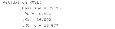
return evaluator.evaluate(dataset)Now we calcuate the training, validation and test RMSE of our baseline model.
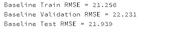
So, we have baseline RMSE for the three datasets. Lets see if we can do better via linear regression, training a model via gradient descent.
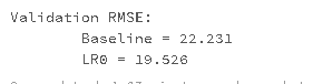
Clearly we have done better than the baseline model, but now we see if we can do better by adding an intercept using regularization and training more iterations. We use LinearRegression to train model with elastic net regularization and an intercept.
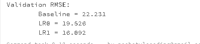
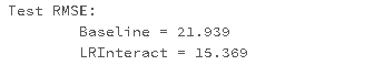
We're already outperforming the baseline on the validation set. Now we perform grid search to find a good regularization parameter and then calculate RMSE. As expected it does a slightly better job.
Once we evaluated our model on validation set we evaluate it on the test data and create the ML pipeline.
pipeline = Pipeline(stages=[polynomial_expansion, linear_regression])
pipeline_model = pipeline.fit(parsed_train_data_df)

predictions_df = pipeline_model.transform(parsed_test_data_df)

evaluator = RegressionEvaluator()
rmse_test_pipeline = evaluator.evaluate(predictions_df, {evaluator.metricName: "rmse"})
Project is hosted on github repository and can be found here